Assessing the accuracy of our solutions¶

If we make the same policy rule plot using EulerIteration.m as we did in VFI.m we find the following

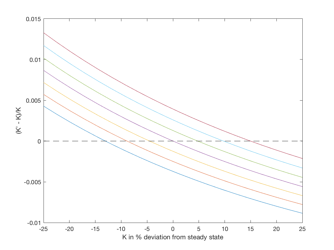
If you compare these to those for VFIHoward.m you will notice that these are convex while those for VFIHoward.m are concave. We have used two methods to solve the same model and we should get the same answer so something must be wrong here.

Actually both solutions are wrong in the sense that they are approximations to the true solution. Some error is unavoidable so our goal is not to eliminate error entirely, but to gain a sense of how accurate our solution is and make sure it is accurate enough for the analysis we are doing.

Inaccuracies arise for two main reasons: numerical errors and programming mistakes. In principle we can find programming mistakes and eliminate them but doing so requires that we put effort to test our code because not all programming mistakes will result in obvious problems like the program crashing. One way of finding programming mistakes is to solve the model in a special case where we know the solution. Another way is to solve the model with different methods and compare the results. I joke that I often have to solve a model three times, because I solve it twice and get different answers and then solve it a third time to figure out where the mistake is. It is important to put just as much care into the test code as the production code. It is easy to fall into the trap of writing sloppy test code (after all it is only a test) only to have the test fail and spend hours looking for a bug in the production code.

We have already done one test: we have solved the same model with value function iteration and by iterating on the Euler equation. And as we saw, the results were not identical to say the least. So what do we do now? My first hypothesis was that the value function algorithm is less accurate than the Euler equation algorithm because we use one degree of our approximate polynomial approximating the intercept of the value function, which has no effect on the consumption-savings choice. To investigate this, I changed the polynomial interpolation scheme in the value function iteration algorithm to allow for more curvature, in particular I added a seventh basis function equal to \(K^3\). When I run VFIHoward.m now, I get something much closer to the results of EulerIt.m. The following figure plots the two sets of results on the same figure.

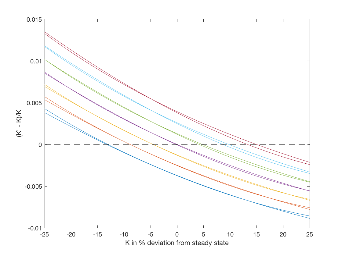
While the two sets of policy rules are not identical, they are much more similar now. From this test, I took away that my hypthosis had been confirmed and if I am going to use value function iteration I need a richer set of basis functions. I still don’t know that the EulerIt.m solution is accurate, but I have some confidence because the two algorithms give very similar results.

Euler equation errors¶

One way of assessing accuracy is to compute the residuals in the equilibrium conditions. Our Euler equation iteration algorithm seeks a set of polynomial coefficients for the approximate consumption function so the equilibium conditions will be satisfied on our grid. As we have 140 grid points and only six polynomial coefficients, we do not have the degrees of freedom to match the function value at all of the grid points. Moreover, we are also intersted the accuracy of our algorithm at points in the state space that are not on the grid and we have no reason to think the equilibrium conditions will be exactly satisfied at those points.

We already have a function, EulerRHS, that calculates the consumption implied by the right-hand side of the Euler equation. For the left-hand side of the Euler equation we can compute consumption directly from the approximate policy rule. We compare these two values to assess the “Euler equation error.”

Suppose our consumption function is approximated by polynomial coefficients bC. We can then proceed as follows:

function Accuracy(Par,Grid,bC)
  TestGrid = Grid;
  TestGrid.nK = 200;

  TestGrid.K = linspace(Grid.K(1),Grid.K(end),TestGrid.nK);
  [Ztest,Ktest] =meshgrid(Grid.Z,TestGrid.K);
  TestGrid.KK = Ktest(:);
  TestGrid.ZZ = Ztest(:);


  C = PolyBasis(TestGrid.KK,TestGrid.ZZ) * bC;
  Kp = f(Par,TestGrid.KK,TestGrid.ZZ) - C;
  CEuler =  EulerRHS(Par,TestGrid,Kp,bC);

  plot(100*(TestGrid.K/Par.Kstar-1), reshape(  log10(abs ( CEuler./C-1 )), 200,7) )
  ylim([-7 -2])
  xlabel('K in % deviation from steady state')
  ylabel('Absolute Euler equation error, log base 10')

We start by creating a new grid structure that will have many more points for capital so we are sure to get a good sense of the errors away from the levels of capital in the grid we used to solve the problem. We could also create a finer grid for \(Z\), but that would involve a little more work to evaluate the Euler equation so we don’t do it here. We then compute two values for consumption. C is computed directly from the approximate policy rule and CEuler is computed from the right-hand side of the Euler equation. We then plot the absolute percentage difference in terms of log base 10.

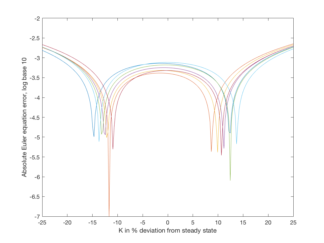
After running VFIHoward we can calculate the consumption function and plot the Euler equation errors as follows:

bC = PolyGetCoef(Grid.KK,Grid.ZZ,f(Par,Grid.KK,Grid.ZZ)-Kp);
Accuracy(Par,Grid,bC)

After running EulerIteration we only need to call

Accuracy(Par,Grid,b)

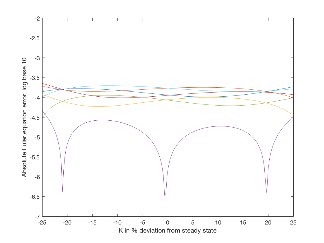
The two figures make clear that the results of EulerIteration have smaller Euler equation errors than VFIHoward. In particular the maximium error plotted for the former is around -3.6 while for the latter it is around -2.7.

The Euler equation error has no units because it is the ratio of consumption over consumption. It can be interpretted as the magnitude of the mistake in percentage terms. So an Euler equation error of \(10^{-3.6}\) is an error of 2.5 dollars per ten thousand spent. For most applications an error of that magnitude would not appreciably alter the conclusions of the analysis. However, we still need to be cautious because even if the Euler equation errors appear small, they only refer to the error in one step of the solution and we cannot rule out that they accumulate to a large inaccuracy over a number of periods.