Stationary Equilibrium of Production Economy
Now let’s extend our model to general equilibrium of a production economy as in Aiyagari (1994). Instead of being endowed with income, let’s say the consumer is endowed with random amounts of labor (efficiency units) that are sold at wage \(W\) per efficiency unit. So now the household budget constraint is
\[a' + c = R a + W e,\]
where now we interpret \(e\) as the labor endowment.
- Production takes place within a representative firm according to the production function
- \[Y = F(K,L) = K^\alpha L^{1-\alpha}.\]
During production, the capital depreciates by amount \(\delta K\). The first order conditions of the firm’s problem are
\[ \begin{align}\begin{aligned}R = \alpha \left( \frac{K}{L} \right)^{\alpha -1} + 1 - \delta\\W = (1-\alpha) \left( \frac{K}{L} \right)^{\alpha}\end{aligned}\end{align} \]
- The aggregate supply of capital comes from the savings of the households so we have
- \[K = \int a_i di = \int a d \Gamma(a,e),\]
where \(\Gamma(a,e)\) is the distribution function over household states. Similarly, the aggregate supply of labor is given by
\[L = \int e_i di = \int e d \Gamma(a,e).\]
\(L\) will be determined by the ergodic distribution of the process for \(e\) and can be calculated separately from the rest of the model.
In specifying the model, the last step is to explain where the distribution \(\Gamma\) comes from. In a stationary equilibrium, the distribution of wealth is the one that recreates itself when households follow the equilibrium savings rule \(g\) and are subjected to the income shocks drawn from \(\Pi(e'|e)\). Mathematically,
\[\Gamma(\mathbb A, e') = \sum_e \left[ \Pi(e'|e) \int_{\{a :g(a,e) \in \mathbb A \} } d \Gamma(a,e) \right]\]
for any set of asset holdings \(\mathbb A\).
In practice we find the stationary distribution \(\Gamma\) by simulating a population of households and the standard algorithm for computing such an equilibrium is as follows
Compute L from the stationary distribution of \(e\)
Guess K
Compute R and W from the firm first order conditions
Solve the household problem to get the decision rule \(g\)
Simulate a population of households to find the candidate \(\Gamma\)
Compute the implied aggregate capital holdings
If the implied capital holdings match the initial guess, stop. Otherwise, update the guess and repeat.
Non-Stochastic Simulation
To simulate a population of households we could use one of several approaches. For the work that comes later it will be useful to use a particular version of non-stochastic simulation. The broad idea is to approximate \(\Gamma(a,e)\) with two histograms corresponding to the continuous distributions of \(a\) associated with the two values of \(e\). To do so we can use the same grid \(A\) of \(N_A\) points that we used in the endogenous grid method. Then let \(D_j\) for \(j\in\{1,2\}\) be a vector of length \(N_A\) that gives the mass of households on the histogram nodes \(A\) for each value of \(e_j\). These two vectors \(\{D_j\}_{j=1}^2\) then represent \(\Gamma(a,e)\).
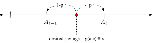
A small challenge with this approach is that the policy rule \(g(a,e)\) will not necessarily select values on the grid. Therefore we need a method of allocating households to grid points near their intended level of savings. To do so we use the guiding principle that the algorithm should preserve the aggregate level of savings. Suppose a unit mass of households have states \((a,e)\) such that the decision rule selects a level of savings \(x\) where \(A_{\ell-1} \leq x < A_{\ell}\) then we will allocate a share \(p\) of this mass to \(A_{\ell}\) and a share \(1-p\) of the mass to \(A_{\ell-1}\) such that \((1-p)A_{\ell-1} + p A_{\ell} = x\). This logic is summarized in the figure below.
Let \(D\) without subscript represent the two vectors \(D_j\) stacked on top of one another. Then we can create a \(2N_A \times 2N_A\) transition matrix that updates the distribution \(D\) according to \(D' = T D\). We create \(T\) column by column. For each pair of current state variables corresponding to a row in \(D\) we fill in four elements of \(T\) corresponding to the two adjacent savings levels that the decision rule maps into according to the previous paragraph crossed with the probabilities of the two possible realizations of next period’s labor productivity.
The stationary distribution of wealth is then the ergodic distribution of the Markov chain \(T\), which is given by the Eigen-vector of \(T\) associated with the unit Eigen-value normalized to sum to one.
Further Implementation Details
We can add the details of our approximate savings policy rule to the logic of how we create the transition matrix \(T\). These are details that you may wish to skip on a first reading. Fix the current states \((a,e)\) and assume we have previously solved for the decision rule in terms of the matrix \(G\). We will focus on a single value of \(e\) and the relevant column of \(G\) so we can think of \(G\) as a vector in what follows. Let \(i\) be the integer such that \(G_{i-1} \leq a < G_{i}\). Let \(x = g(a,e)\) be the level of savings at \((a,e)\). This can be calculated from our linear interpolation scheme as
\[x = \frac{A_{i}-A_{i-1}}{G_{i}-G_{i-1}}\left(a - G_{i-1} \right) + A_{i-1}\]
- as shown in the following figure.
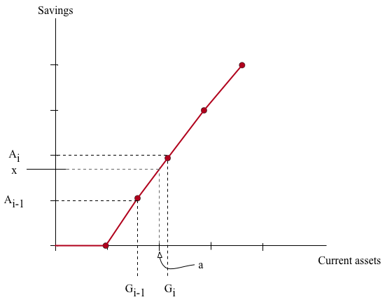
Notice that in this interpolation scheme we will have \(\ell = i\). Using the logic above, we assign a share \(p = (x-A_{i-1})/(A_{i}-A_{i-1})\) of the mass that started at \((a,e)\) to the future savings level \(A_{i}\) and a share \(1-p\) to the savings level \(A_{i-1}\). Putting the two steps together we have
\[p = \frac{a - G_{i-1}}{G_{i}-G_{i-1}}\]
We then use the following algorithm to construct the transition matrix \(T\):
Set \(T\) to a square matrix of zeros of size \(2N_A \times 2N_A\).
- Loop over \(e_j\) for \(j\in\{0,1\}\) and let \(G\) be the vector representing the corresponding decision rule.
Let \(s = jN_A\).
- For each \(A_m \in A\) look up \(A_m\) in the vector \(G\) and define \(i\) such that \(G_{i-1} \leq A_m < G_{i}\).
Set \(p = \frac{A_m - G_{i-1}}{G_{i}-G_{i-1}}\).
Set
\[ \begin{align}\begin{aligned}T_{i,s+m} &= \Pi(e_0|e_j) p\\T_{i-1,s+m} &= \Pi(e_0|e_j) (1-p)\\T_{N_A + i,s+m} &= \Pi(e_1|e_j) p\\T_{N_A + i-1,s+m} &= \Pi(e_1|e_j) (1-p)\end{aligned}\end{align} \]