Endogenous Grid Method
Consider a consumer facing fluctuating income \(e\) that follows a Markov chain with transition probabilities \(\Pi(e'|e)\) where a prime denotes next period’s value of a variable. To keep things simple, we will assume that \(e\) takes two values. The consumer can save in a risk-free bond at return \(R\). The budget constraint is therefore
\[a' + c = R a + e,\]
- where \(a\) is assets before interest. Let’s suppose that there is a borrowing constraint \(a' \geq 0.\) The consumer wishes to maximize a utility function of
- \[\mathbb E_0 \sum_{t=0}^\infty \beta^t \frac{ c_t^{1-\gamma}}{1-\gamma}\]
The states of the consumer’s problem are \((a,e)\) and so a solution to this problem can be represented as a function \(g(a,e)\) that gives the choice of \(a'\).
- We will solve this problem using the Euler equation
- \[c^{-\gamma} = \beta R \mathbb E \left[ {c'}^{-\gamma} \right],\]
- where the expectation is taken over values of \(e'\). Given the savings policy rule we can use the budget constraint to find the consumption function
- \[c(a,e) = R a + e - g(a,e).\]
The heart of the endogenous grid method is as follows. Suppose this period we have states \((a,e)\) where we know \(e\), but as of yet we don’t know \(a\). Suppose we save an amount \(A\) so we have \(g(a,e) = A\) and we will have to determine \(a\). Then the Euler equation can be written as
\[c(a,e)^{-\gamma} = \beta R \mathbb E_{e'} \left[ \left\{R A + e' - g(A,e')\right\}^{-\gamma} \right].\]
Given a guess of the policy rule \(g\) we can compute the right-hand side and solve this equation for \(c(a,e)\). Next we use the budget constraint to solve for \(a\)
\[a = \frac{1}{R}\left[ c(a,e) + A - e \right].\]
We now have a new policy rule that maps \((a,e)\) to \(A\). We use this as our new guess of the function \(g(a,e)\) and repeat these steps until the algorithm converges meaning the guess of \(g\) reproduces itself upto some small discrepancy.
Implementation concepts
We now discuss some of the details of how we implement these ideas.
Approximating the decision rules
A function cannot itself be represented in a computer so the first decision we have to make is how to approximate the savings policy rule. We will do this in a somewhat counter-intuitive way that turns out to simplify the problem. This approach assumes that the policy rule is strictly increasing in \(a\) when the borrowing constraint doesn’t bind.
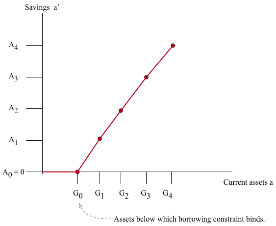
Let \(A\) be a grid of \(N_A\) points on values of \(a'\) with the first gridpoint at the borrowing constraint, zero in this case. Now let \(G\) be a \(N_A \times 2\) matrix where each column is a strictly increasing vector of length \(N_A\) that represents the policy rule as a function of \(a\) for one of the values of \(e\). The interpretation now is that if you have states \((G_{i,j},e_j)\) then the policy rule calls for saving \(A_i\). For values of \(a\) between two values of \(G_{i,j}\) and \(G_{i+1,j}\) we will use linear interpolation to fill in the function.
- The following figure summarizes our function approximation scheme. The grid \(A\) is fixed on the vertical axis and the function is approximated by choosing the values \(G\) on the horizontal axis.
A projection method interpretation
The endogenous grid method is generally used as an iterative algorithm in which one guesses a policy rule and the algorithm provides the next candidate policy rule (if the two agree within some tolerance the algorithm stops). In solving models with aggregate shocks, it is useful to give the endogenous grid method an interpretation as a projection method. In this interpretation, we approximate the policy rules with the vector \(G\) and we then ask if a candidate \(G\) solves the Euler equation at a set of points. We could search over \(G\) to find the policy rule that solves the household’s problem although we will not do that exactly.
To this end, let’s define a function \(g(a,e;G)\) that gives savings at state \((a,e)\) when the policy rule is parameterized by \(G\). This function is constructed from the interpolation logic described above. Next, let’s define the function \(c(a,e;G)\) that gives consumption in state \((a,e)\) when the policy rule is parameterized by \(G\). This function can be solved from the budget constraint: \(c(a,e;G) = R a + e - g(a,e;G)\). Next define the function \(\mathcal C (a,e;G)\) from the right-hand side of the Euler equation when savings are \(A\)
\[\mathcal C (A,e;G) = \left\{ \beta R \mathbb E_{e'} \left[ c(A,e';G)^{-\gamma} \right] \right\}^{-\frac{1}{\gamma}}.\]
If the Euler equation holds for the policy rule parameterized by \(G\), then \(\mathcal C (A,e;G)\) should be equal to \(c(g^{-1}(A,e;G),e;G)\) where \(g^{-1}(A,e;G)\) is the inverse of the \(g\) function (i.e. the level of current assets \(a\) that leads to savings \(A\).)
Now, let’s fix the grid \(\{A\}\) for savings as in the interpolation scheme. Note that in this case \(g^{-1}(A_i,e_j;G)\) is \(G_{i,j}\). We can then express Euler equation residuals as
\[R(A_i,e_j;G) \equiv \frac{\mathcal C (A_i,e_j;G)}{c(G_{i,j},e_j;G)} - 1\]
for each \(i\) and \(j\). \(R=0\) is a system of equations of a size conformable to the shape of \(G\) that holds at the solution for \(G\).