Setting up the problem¶

We are now ready to solve the model using our first method, which is value function iteration. To do so, we are going to have to set up the model in the computer, by which I mean we are going to tell the computer what we know about the problem. We can begin as follows:

% Store the parameters in a structure
Par.beta = 0.99;
Par.gamma = 2;
Par.alpha = 0.36;
Par.delta = 0.03;
Par.rho = 0.95;
Par.sigma = 0.007;


%% Solve for the steady state
Zstar = 0;
Kstar = ((1/Par.beta - 1 + Par.delta)./(Par.alpha * exp(Zstar))).^(1/(Par.alpha-1));

We store the parameters in a Matlab structure, which is a grouping of variables. This might seem like extra work but it will be useful because then we can pass the whole structure to a function instead of having to specify all of the individual variables. We then solve for the steady state capital stock from the equation

\[f'(K^*) = 1/\beta.\]

The next step is to set up our grid on \(K\) and \(Z\). This grid needs to cover a two-dimensional space so we are going to create two one-dimensional grids and then take the Cartesian product of the two.

%% Create a grid for Z
meanZ = 0;
Grid.nZ = 7;  % number of points in our grid for Z
numStdZ = 2;  % number of standard deviations to cover with the grid
[Grid.Z, Grid.PZ]  = tauchen(Grid.nZ, meanZ, Par.rho, Par.sigma, numStdZ);

Grid.PZ = Grid.PZ'; % this is a 7 x 7 transition matrix for which the columns sum to 1
% the (i,j) element is the probability of moving from j to i.

To create the grid for \(Z\) and the transition matrix we use an implementation of the Tauchen method. We discussed this above and we won’t go further into the details here. We create a Grid structure to hold all of our variables associated with the grids.

%% Create a grid for K
Grid.nK = 20;
Grid.K = linspace(0.75*Kstar, 1.25*Kstar,Grid.nK)';  % this is a 20 x 1 array of evenly spaced points

The grid for \(K\) is made up of a set of 20 evenly spaced points that extends from 25 percent below the steady state to 25 percent above.

%% Create a product of the two grids
[ZZ,KK] =meshgrid(Grid.Z,Grid.K);
Grid.KK = KK(:);
Grid.ZZ = ZZ(:);

The Matlab function meshgrid creates the Cartesian product of two vectors. The output of meshgrid is two 20 x 7 arrays with KK(i,j) equal to K(i) and ZZ(i,j) equal to Z(j). The next line unravels the array KK into a single column and stores it in the Grid structure. The use of the colon operator (:) means treat the elements of this array as a single column regarless of the shape of the array. The last line unravels ZZ in the same way.

How does Matlab store and reference arrays?¶

A small detour about how Matlab stores arrays. Suppose you create the array

A = [1 2;
     3 4;
     5 6]

This is an array with three rows and two columns. If we type A(:) we find

>> A(:)

ans =

   1
   3
   5
   2
   4
   6

Notice that Matlab reads down the columns first and then down the rows. This works the other way around, too. If we create a vector and reshape it into an array, Matlab will fill the array up the column by column

>> A = 1:4

A =

     1     2     3     4

>> reshape(A,2,2)

ans =

     1     3
     2     4

The Bellman operator¶

We now code the Bellman equation into the computer and we do this in two steps. First, we write a function that evaluates the right hand side of the Bellman equation for a given choice of \(K'\). Second, we write a function that will maximize the right hand side of the Bellman equation. Before we begin, it will be convenient to have a function that evaluates our production function \(f(K,Z)\).

function y  = f(Par, K,Z )
% y  = f( K,Z )
%   Production function gross of undepreciated capital

y =  exp(Z) .* K.^Par.alpha + (1-Par.delta)*K;
end

Next we code the Bellman equation given a level of savings.

function V  = Bellman( Par, b, K, Z, Kp )
% V  = Bellman( Par, b, K, Z, Kp )
%   Evaluate the RHS of the Bellman equation
%
% Inputs
% Par   Parameter structure
% b     6 x 1 coefficients in polynomial for E[ V(K',Z') | Z ]
% K     n x 1 array of current capital
% Z     n x 1 array of current TFP
% Kp    n x 1 array of savings
%
% Output
% V     n x 1 array of value function
%

C = f(Par,K,Z) - Kp;
u = C.^(1-Par.gamma) / (1-Par.gamma);
V = u + Par.beta * PolyBasis(Kp,Z) * b;



end

The first line calculates consumption from the resource constraint and the next line computes the period utility from that consumption. The third line creates the output variable V equal to the sum of the period and continuaion utilities.

Notice that we are not actually going to approximate the value function but rather we are approximating \(\mathbb E \left[ V \left( K' ,Z' \right) | Z \right]\). Therefore the function we are approximating is a function of how much we save \(K'\), which is known today, and the current level of TFP \(Z\). To evaluate that function we create our polynomial basis matrix and then multiply it against the coefficients of our polynomial.

Notice that the Bellman function takes the level of savings as an input, but the Bellman equation involves maximizing over this choice variable. We can now do the maximization in the Bellman equation using golden section search and we will create a function to do this.

function [V, Kp] = MaxBellman(Par,b,Grid)
% [V, Kp] = MaxBellman(Par,b,Grid)
%   Maximizes the RHS of the Bellman equation using golden section search
%
% Inputs
% Par       Parameter structure
% b     6 x 1 coefficients in polynomial for E[ V(K',Z') | Z ]
% Grid      Grid structure


p = (sqrt(5)-1)/2;

A = Grid.K(1) * ones(size(Grid.KK));
D = min(f(Par,Grid.KK,Grid.ZZ) - 1e-3, Grid.K(end)); % -1e-3 so we always have positve consumption.

B = p*A+(1-p)*D;
C = (1-p)*A + p * D;


fB = Bellman(Par,b,Grid.KK,Grid.ZZ,B);
fC = Bellman(Par,b,Grid.KK,Grid.ZZ,C);


MAXIT = 1000;
for it_inner = 1:MAXIT

    if all(D-A < 1e-6)
        break
    end

    I = fB > fC;

    D(I) = C(I);
    C(I) = B(I);
    fC(I) = fB(I);
    B(I) = p*C(I) + (1-p)*A(I);
    fB(I) = Bellman(Par,b,Grid.KK(I),Grid.ZZ(I),B(I));

    A(~I) = B(~I);
    B(~I) = C(~I);
    fB(~I) = fC(~I);
    C(~I) = p*B(~I) + (1-p)*D(~I);
    fC(~I) = Bellman(Par,b,Grid.KK(~I),Grid.ZZ(~I),C(~I));

end

% At this stage, A, B, C, and D are all within a small epsilon of one
% another.  We will use the average of B and C as the optimal level of
% savings.
Kp = (B+C)/2;

% evaluate the Bellman equation at the optimal policy to find the new
% value function.
V = Bellman(Par,b,Grid.KK,Grid.ZZ,Kp);

end

We start by defining the constant \(p\) for the golden section search. We then specify the interval of \(K'\) that we will search over and we will assume that we never leave the grid on the low side and we never save so much as to have negative consumption on the high side and we will never save so much as to leave the grid. Notice that these are vectors that corresond to the size of our grid vectors KK and ZZ. We then define the points B and C using the golden section ratios and evaluate the Bellman function at those points. Notice that everything we are doing here is operating on vectors of \(K'\) that correspond to the choices at the corresponding levels of \(K\) and \(Z\) that appear in Grid.KK and Grid.ZZ.

Next we enter a loop for 1,000 iterations. We will continue shrinking the interval until the distance between D and A is sufficiently small as shown in the first lines of the loop code. The comparison D - A < 1e-6 will generate a logical array (an array of true and false values) that checks the distance between each element of D and each corresponding element of A. The all function will then tell us whether all of the values in the logical array are true. The break command tells the program to leave the loop it is executing. One could use a while loop for this, but a danger with that approach is that if there is a bug the program could run forever in a while loop whereas with the for loop it will stop after MAXIT iterations at most.

The next part of the algorithm is a little tricky. When we discussed golden section search we were maximizing a scalar function with respect to a single argument. But in this application we are maximizing different functions (if we think of the variation in the rows of Grid.KK and Grid.ZZ giving rise to different Bellman functions for Kp) with respect to a vector of values Kp. Each row can be considered a scalar function of a scalar argument but we are doing many independent maximizations at the same time. In this case we won’t necessarily find that fB > fC for all of the rows, nor vice versa. So we define an indicator function or “logical array” for whether fB > fC. In the lines that follow we will first do the operations for those rows for which the logical array is true and then we will do the operations for which the rows are false using ~I because the ~ inverts the logical values in the array. In either case the operations are straightforward. For the cases for which fB > fC we are going to eliminate the interval \(CD\) so for these rows \(C\) becomes the new \(D\) which we accomplish with D(I) = C(I) then \(B\) becomes the new \(C\) which we accomplish with C(I) = B(I) and the function values at \(B\) become the function values at \(C\) which we accomplish with fC(I) = fB(I). Next we create a new \(B\) and evaluate the function at those points. The remaining block of code performs the analogous operations for the cases fB < fC where we eliminate the interval \(AB\).

After we have exited the loop, we just have a little more work to do. By construction, A, B, C, and D are all within 1e-6 of one another so we will take the average of B and C and treat it as the true maximizer Kp. Next we evaluate the Bellman function at Kp to get the maximized value.

Updating our guess of the value function¶

Our MaxBellman function takes the coefficients b of our approximate value function as an argument, but we don’t yet know what those are because we don’t know the value function before we have solved for it. The idea of value function iteration is that we can start with any value function and apply the Bellman operator repeatedly to iterate towards the true value function. So we need a guess of the value function to start with. We will do something naive and guess that it is the zero function meaning expected value is also the zero function and the coefficients of our approximating polynomial are all zero.

b = zeros(6,1);

After applying MaxBellman we have a vector of values that give us \(V(K,Z)\) on our grid for \(K\) and \(Z\). But this value function was calculated for a given guess of b or equivalently a guess of \(\mathbb E \left[ V \left( K' ,Z' \right) | Z \right]\), which was not necessarily the true expected continuation value. Now we are going to use our new \(V(K,Z)\) to update our guess of \(\mathbb E \left[ V \left( K' ,Z' \right) | Z \right]\). To do so is easy given that we have already done the work of discretizing our AR(1) process for \(Z\).

The first step is to reshape V into a 20 by 7 array where the rows correspond to different levels of capital and the columns correspond to different levels of TFP. Because we were a little bit clever in how we set up the arrays Grid.KK and Grid.ZZ, this is just a matter of calling Matlab’s reshape command like this reshape(V,Grid.nK,Grid.nZ). So a given row of this array is the value function at the same level of capital but at different levels of TFP. To compute the conditional expectation conditional on the previous level of TFP, we just need to take the dot product of this row of the array with the appropriate column of the Markov chain transition matrix. We can get all of the conditional expectations with a matrix multiplication like this

EV = reshape(V,Grid.nK,Grid.nZ) * Grid.PZ;

EV is an array where each row corresponds to \(K_t\), each column corresponds to \(Z_{t-1}\) and the entires are \(\mathbb E \left[ V( K_t, Z_t) | Z_{t-1} \right]\).

Now that we have computed the expected value on our grid, we can update the coefficients of the polynomial that approximates this function using the PolyGetCoef function that we wrote earlier.

b1 = PolyGetCoef(Grid.KK,Grid.ZZ,EV(:));

We use (:) to unravel the EV array into one column that matches the layout of Grid.KK and Grid.ZZ.

Putting the iteration in value function iteration¶

We have now completed one step in our algorithm. We started with a guess of the value function polynomial coefficients and we arrived at a new set of coefficients. We are now going to repeat the process many times over using a for loop until the value function has converged.

How do we know when to stop? A good approach is to check for convergence in terms of something that you actually are interested in. So instead of checking that the polynomial coefficients have converged, let’s check that the policy rule has converged. To do that, let’s introduce a copy of the previous policy rule, call it Kp0 and compare the new policy rule to it.

Kp0 = zeros(size(Grid.KK));
MAXIT = 2000;
for it = 1:MAXIT

    [V, Kp] = MaxBellman(Par,b,Grid);


    % take the expectation of the value function from the perspective of
    % the previous Z
    EV = reshape(V,Grid.nK,Grid.nZ) * Grid.PZ;

    % update our polynomial coefficients
    b = PolyGetCoef(Grid.KK,Grid.ZZ,EV(:));

    % see how much our policy rule has changed
    test = max(abs(Kp0 - Kp));
    Kp0 = Kp;

    disp(['iteration ' num2str(it) ', test = ' num2str(test)])
    if test < 1e-5
        break
    end
end

Results!¶

We now have all of the pieces we need solve for the value function and policy rule using value function iteration. If you run the script VFI.m you should see your computer iterate for about 200 iterations.

Now that we have solved the problem, we can look at the results. The following commands make a plot of the policy rules

DK = Grid.K/Kstar-1; % Capital grid as percent deviation from steady state

DKp = reshape(Kp,Grid.nK,Grid.nZ)./reshape(Grid.KK,Grid.nK,Grid.nZ) - 1;
  % savings policy rule as a 20 x 7 array expressed as a percent change from current K

plot(DK, DKp);  % plot the policy rule

hold on;        % next plots go on the same figure

plot(DK, zeros(Grid.nK,1), 'k--'); % add a zero line, k-- means black and dashsed

xlabel('K in % deviation from steady state')  % label the axes
ylabel('(K'' - K)/K')

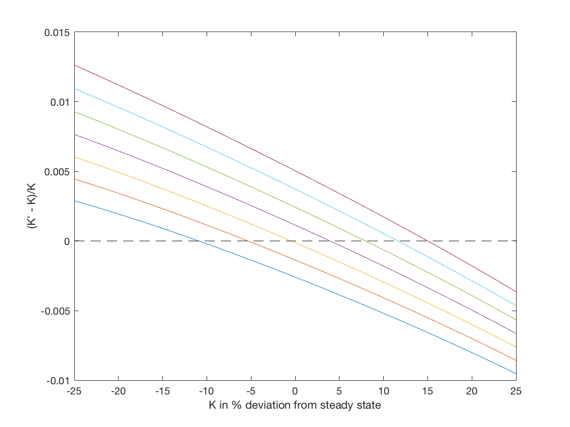
The horizontal axis is the current capital stock as a percentage difference from the steady state and the vertical axis is the next period’s capital stock as a percentage difference from this period’s. There are seven lines on the figure corresponding to the different levels of current TFP. The lowest line corresponds to the lowest TFP and so on. As you can see, if current capital is low enough then the optimal policy is to increase the capital stock for all TFP levels and if the current capital is high enough then the optimal policy is to eat down the capital stock for all TFP levels. In between, the optimal policy is to build capital if TFP is high and reduce capital if TFP is low.

Suppose now we want to know the optimal policy at a point not on our grid. We can use interpolation to infer this from the value that we computed on the grid.

bKp =  PolyGetCoef(Grid.KK,Grid.ZZ,Kp);
Kp2903 = PolyBasis(29,0.03) * bKp
C2903 = f(Par,29,0.03) - Kp2903

First we fit a polynomial to the policy rule and then we evaluate that polynomial at the point \(K = 29\) \(Z = 0.03\) to get the interpolated savings at that point. Finally we can use the aggregate resource constraint to find consumption at that point.

Going faster¶

If you run the program VFI.m it should take a couple of seconds to run. You can time it by typing

tic; VFI; toc

at the Matlab command prompt which will tell Matlab to start a timer before running the program and then report the elapsed time at the end of the program. While this might not seem like a long time to wait, this model is just about the simplest dynamic programming problem we could come up with. Modern macro models can involve many state variables, many choice variables, and many shocks all of which increase the computational burden. In fact, as the number of state variables rises, the number of combinations of states we have to consider rises exponentially so the computational burden of solving the model grows very quickly as the number of state variables increases. This issue is known as the “curse of dimensionality.” To illustrate, in this application we had two state variables and we put a grid of 20 points on capital and a grid of 7 points on productivity, which resulted in 140 points in our product grid (Grid.KK,Grid.ZZ). Now suppose we had a a model with two countries each with their own capital stock and productivity. If we created the grid in the same way, we would have \(20\times7\times20\times7=19600\) points in our grid so computing a solution would not twice as long but roughly 140 times as long! Things are not so dire as this suggests: first, we can speed up our algorithm with a small tweak we will discuss now, second we can use a different even faster algorithm, third there are ways of limiting the curse of dimensionality by choosing the grid in a more clever way than just taking the product of one-dimensional grids, for example here or here.

A simple change to our value function iteration algorithm will make it run much faster. This technique is known as “Howard acceleration”. When I ran VFI.m and it took 4.1 seconds and 3.6 of those seconds were spent in the MaxBellman function. So our goal is to reduce the time spent in MaxBellman. The value function depends on the policy rule(s) we will use at all future dates. In the value function iteration algorithm we are only slowly incorporating the new policy rule that emerges from our maximization into the value function because the continuation value still depends on the initial guess of the value function and implicitly then depends on sub-optimal policy rules. Instead of just iterating the Bellman equation, we could find the optimal policy rule and then find the value function that is implied by following that policy rule and then iterate the Bellman equation again. By doing this, we would be incorporating the new policy rule into the value function much more quickly. A simple change to our VFI.m program will incorporate this idea and give us a considerable speedup. Instead of finding the optimal policy rule at each iteration, we can iterate the Bellman equation for several hundred iterations using the same policy rule. This updates the value function much more for each policy rule and reduces considerably the number of times we need to do the costly maximization.

VFIHoward.m differs from VFI.m in the following way

Kp0 = zeros(size(Grid.KK));
MAXIT = 8000;
for it = 1:MAXIT

    if mod(it,500) == 1
        [V, Kp] = MaxBellman(Par,b,Grid);

        % see how much our policy rule has changed
        test = max(abs(Kp0 - Kp));
        Kp0 = Kp;
        disp(['iteration ' num2str(it) ', test = ' num2str(test)])
        if test < 1e-5
            break
        end
    else
        V = Bellman(Par,b,Grid.KK,Grid.ZZ,Kp);
    end

    % take the expectation of the value function from the perspective of
    % the previous Z
    EV = reshape(V,Grid.nK,Grid.nZ) * Grid.PZ;

    % update our polynomial coefficients
    b = PolyGetCoef(Grid.KK,Grid.ZZ,EV(:));


end

In this algorithm, we only call MaxBellman and update the policy rule every 500th iteration. In the other iterations we just update the value function by calling the Bellman function with the existing (not necessarily optimal) policy rule. We will need to do more iterations overall, so we increase MAXIT, but only a small fraction of them will involve the costly maximization. Running VFIHoward.m takes 1.0 seconds and only 0.1 seconds are spent doing the maximization.