Numerical maximization
- In the Bellman equation we maximize over \((C,K')\). By substituting the aggregate resource constraint we can phrase this as a maximization over one choice variable
- \[\begin{split}V(K,Z) &= \max_{K'} \left\{ u\left( f(K,Z) - K' \right) + \beta \mathbb E V(K',Z') \right\}.\end{split}\]
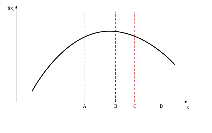
Optimization is a large field of numerical analysis, but in these notes we will consider just one method that is easy to understand and fairly robust called “golden section search”. Suppose we have a function \(F(x)\) and we want to maximize it on the interval \([\underline{x},\bar x]\). We start by evaluating the function at four points labeled \(A\), \(B\), \(C\), and \(D\) in the following diagram.

To start with we would set \(A = \underline{x}\) and \(D = \bar x\). We then observe that \(F(C)>F(B)\) so we use the following reasoning to discard the interval \([A,B]\) from containing the maximizer: if \(F(x)\) is concave then the derivative is weakly decreasing and if the true maximizer \(x^*\) were in \([A,B]\) then the function goes down from \(x^*\) to B and then up from B to C, which contradicts the supposition that \(f\) is concave. You could use this algorithm if \(f\) is not concave but then there are no guarantees that it will work.
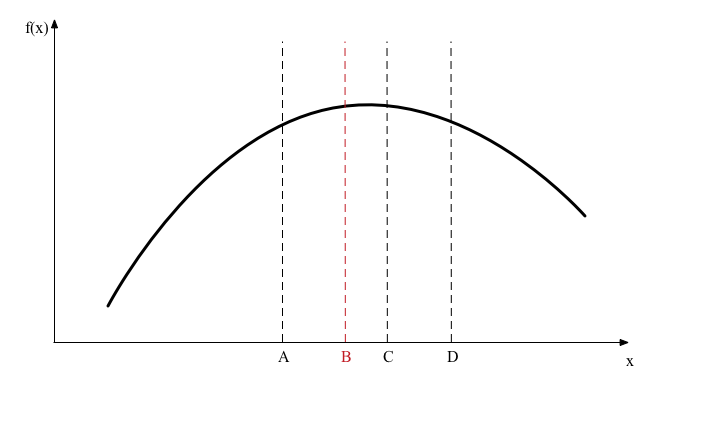
Once we eliminate the interval \([A,B]\) we repeat the same steps on the interval \([B,D]\) that is smaller than our original interval \([A,D]\). So point \(B\) will become the new \(A\). The clever part of the algorithm is that we put the points \(B\) and \(C\) in just the right places so that now \(C\) becomes the new \(B\). This means we don’t need to re-evaluate the function at our new points \(A\) or \(B\). We now introduce a new point \(C\), evaluate the function there and repeat as shown in the next diagram.
In the next iteration we find \(F(B)>F(C)\) so now we discard \([C,D]\), \(C\) becomes the new \(D\), and \(B\) becomes the new \(C\).
As you can see in the diagrams, the region under consideration is shrinking towards the true maximizer. If we repeat this procedure many times over we will have \([A,D]\) tightly bracketing \(x^*\).
Finally, how do we choose the points \(B\) and \(C\)? We are going to impose some symmetry on the choice so the interval \([A,B]\) is the same length as \([C,D]\). This reduces the problem to choosing one number \(p \in (0,1)\) as shown in the following figure.

- We want to choose \(p\) so that when we eliminate \([A,B]\) point \(C\) becomes the new point \(B\) so we need the ratio of \(BC\) relative to \(BD\) to be the same as \(AB\) relative to \(AD\). To accomplish this we need
- \[\frac{2p-1}{p} = 1-p.\]
This equation reduces to a quadratic equation with one root \(p = (-1 + \sqrt{5})/2\). As the other root implies \(p<0\) we disregard it.
Why is the method called “golden section search”? Because \(1/p\) is the golden ratio.